A simple tutorial of developing LSTM model for Time-Series Forecasting

Concept
If you remember the plot of one of the MCU movie series Captain America: The First Avenger, Zola’s Algorithm was created to predict an individual’s future by evaluating their personal information such as bank records, medical histories and etc. Well, if you forgotten…here’s the clip to revise :
https://www.youtube.com/watch?v=tmfLYkcgJD8&ab_channel=GregBurton
In short, the application of Zola’s Algorithm is to predict the future by looking back at the previous data, similar to today’s Recurrent Neural Network (RNN) where it is used to forecast the dependent variables based on previous independent variables.
In this article, I will build a Multivariate Multi-Step predictive model using LSTM algorithm running in Google Colab. If you wish to understand how LSTM work before heading to the coding part, here is an great article with .gif that explain everything :
What is Time-Series Forecasting ?
Time-Series forecasting basically means predicting future dependent variable (y) based on past independent variable (x).
What is Multivariate Forecasting ?
If the model predicts dependent variable (y) based on one independent variable (x), it is called univariate forecasting. For Multivariate forecasting, it simply means predicting dependent variable (y) based on more than one independent variable (x).
What is Multi-step Forecasting ?
If the model predicts a single value for next time-step, it is called one-step forecast. For Multi-step forecast, it means predicting few times-steps ahead.
What is Multivariate Multi-step Time-Series Forecasting ?
With all methods combined, the model in this article will predict multi-step ahead of dependent variable (y) based on the past two independent variables (x).
Full code
Click HERE for full code and all the necessary files.
Begin.
Libraries required
import numpy as np
import matplotlib.pyplot as plt
import pandas as pd
import statsmodels.api as sm
from pandas import DataFrame , concat
from sklearn.metrics import mean_absolute_error , mean_squared_error
%matplotlib inline
%config InlineBackend.figure_format = 'retina'
from numpy import mean , concatenate
from math import sqrt
from pandas import read_csv
from sklearn.preprocessing import MinMaxScaler
from tensorflow.keras.models import Sequential
from tensorflow.keras.layers import Dense,LSTM,Activation
from numpy import array , hstack
from tensorflow import keras
import tensorflow as tf# if you're using google drive to store the dataset
from google.colab import drive
drive.mount('/content/drive')
Dataset
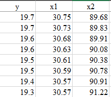
In this project, the dataset contain the independent variables (x1 , x2) and the dependent variables are (y) as shown in the Table below.

Visualize Data
In this dataset, we have total of 28 batches of data containing 1 dependent variable(y) and 2 independent variables(x1,x2). Each variable in every batch contain 1258 data points. Forming 1258 * 28 = 35224 of data points for each variable.
url = '/yourDirectory/Dataset.csv'
dataset = pd.read_csv(url)
x_1 = dataset['x1']
x_2 = dataset['x2']
y = dataset['y']x_1 = x_1.values
x_2 = x_2.values
y = y.valuesplt.figure(figsize=(30, 6))
plt.plot(x_1[:10064] , label='x1')
plt.plot(x_2[:10064] , label='x2')
plt.plot(y[:10064] , label='y')
plt.legend(loc='upper right')
plt.title("Dataset" ,  fontsize=18)
plt.xlabel('Time step' ,  fontsize=18)
plt.ylabel('Values' , fontsize=18)
plt.legend()
plt.show()

Training Data Pre-Processing
In common practice, data are usually pre-processed before splitting into train and test set. Here, we will need to perform data transformation by normalizing each variable data using MinMaxScaler. The steps are as follows :
- reshape each variable to 2D array with the configuration :(number of data, 1) for scaling.
- Specify a Scaler ranging from 0 to 1 and fit each data variable individually. To Note : the fit_transform() function comprises of both function fit() and transform(), where it scan the max and min value of the data and transform them between 0 and 1. If the data has different range, the transformation will be different. For more info : MinMaxScaler()
- Stack all the variables horizontally.
# Step 1 : convert to [rows, columns] structure
x_1 = x_1.reshape((len(x_1), 1))
x_2 = x_2.reshape((len(x_2), 1))
y = y.reshape((len(y), 1))print ("x_1.shape" , x_1.shape)
print ("x_2.shape" , x_2.shape)
print ("y.shape" , y.shape)# Step 2 : normalization
scaler = MinMaxScaler(feature_range=(0, 1))
x_1_scaled = scaler.fit_transform(x_1)
x_2_scaled = scaler.fit_transform(x_2)
y_scaled = scaler.fit_transform(y)# Step 3 : horizontally stack columns
dataset_stacked = hstack((x_1_scaled, x_2_scaled, y_scaled))
print ("dataset_stacked.shape" , dataset_stacked.shape)
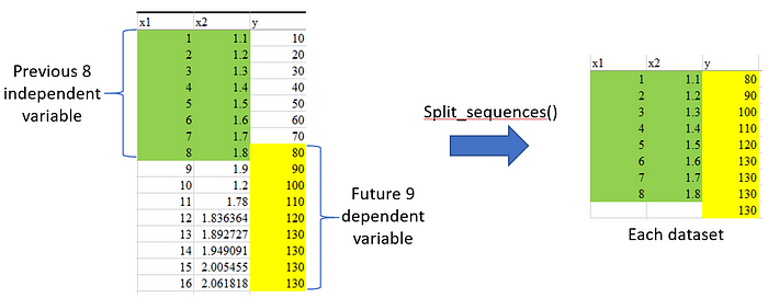
We want our model to learn by relating the previous [x1,x2] data with the future [y] data. Therefore, we need to re-arrange our data accordingly by using a split sequences() function created by MachineLearningMastery. There are 2 key arguments we need to specify which are :
1. n_steps_in : Specify how much data we want to look back for prediction
2. n_step_out : Specify how much multi-step data we want to forecast
Example : given n_steps_in = 8 and n_step_out = 9, the training data will be arrange as per figure below, by arranging 8 independent variable with the next 9 dependent variable (including current step).

In this project, we will lookback on 60 (x1,x2) past data, to forecast future 30 multi-step ahead of data. Therefore, the returned X and y are time-step shifted according to the argument, the the size should be (35139, 60, 2) and (35139, 30).
The returned array are arranged in [n_dataset, n_steps_in , n_features] and [n_dataset, n_steps_out]. Feel free to print it out to understand more by using this code : print(X[i], y[i])
# split a multivariate sequence into samples
def split_sequences(sequences, n_steps_in, n_steps_out):
 X, y = list(), list()
 for i in range(len(sequences)):
  # find the end of this pattern
  end_ix = i + n_steps_in
  out_end_ix = end_ix + n_steps_out-1
  # check if we are beyond the dataset
  if out_end_ix > len(sequences):
   break
  # gather input and output parts of the pattern
  seq_x, seq_y = sequences[i:end_ix, :-1], sequences[end_ix-1:out_end_ix, -1]
  X.append(seq_x)
  y.append(seq_y)
 return array(X), array(y)# choose a number of time steps #change this accordingly
n_steps_in, n_steps_out = 60 , 30# covert into input/output
X, y = split_sequences(dataset_stacked, n_steps_in, n_steps_out)
print ("X.shape" , X.shape)
print ("y.shape" , y.shape)
Splitting Data
As mentioned earlier, we have total of 28 batches of dependent and independent variables, now is the time to split them into 25 batches for training and the rest 3 batches for testing.
split_point = 1258*25
train_X , train_y = X[:split_point, :] , y[:split_point, :]
test_X , test_y = X[split_point:, :] , y[split_point:, :]
Finally, our testing and training data shape should be like this :
train_X.shape (31450, 60, 2) [n_datasets,n_steps_in,n_features]
train_y.shape (31450, 30) [n_datasets,n_steps_out]
test_X.shape (3689, 60, 2)
test_y.shape (3689, 30)
n_features = 2
LSTM Model Setting
Here, we will start to set up our LSTM model architecture by initializing the optimizer learning rate as well as number of layers in the network. The neural network consist of : 2 LSTM nodes with 50 hidden units, a dense layer which specify the model’s output based on n_steps_out (how many future data we want to forecast) and end with an activation function.
To Note : The input_shape of the first LSTM node specify the shape of input data for prediction in the evaluation phase. Meanwhile, the Dense Layer specify the output shape of the model based on n_steps_out
#optimizer learning rate
opt = keras.optimizers.Adam(learning_rate=0.0001)# define model
model = Sequential()
model.add(LSTM(50, activation='relu', return_sequences=True, input_shape=(n_steps_in, n_features)))
model.add(LSTM(50, activation='relu'))
model.add(Dense(n_steps_out))
model.add(Activation('linear'))
model.compile(loss='mse' , optimizer=opt , metrics=['mse'])
Training
In training, we have 25 batches of dataset, therefore the steps_per_epoch will be 25. In each steps, it will take 1258 data points (1 batch) for training. With 25 steps per epoch, all 25 batches will be trained in each epoch. With 60 epochs, each batch will be trained 60 times. The whole training progress should be less than 15minutes with Google Colab.
# Fit networkhistory = model.fit(train_X , train_y , epochs=60 , steps_per_epoch=25 , verbose=1 ,validation_data=(test_X, test_y) ,shuffle=False)
Test Data Preparation
Here, the 3 batches of test data are manually saved in different csv file to ease the evaluation process. First, read the first batch of test data, reshape and scale it.
# Test Data Batch 1 , Test Data Batch 2 , Test Data Batch 3
url_test = '/directory/Test Data Batch 1.csv'
dataset_test_ok = pd.read_csv(url_test)
dataset_test_ok.head()# read test data
x1_test = dataset_test_ok['x1'].values
x2_test = dataset_test_ok['x2'].values
y_test = dataset_test_ok['y'].values # no need to scale# convert to [rows, columns] structure
x1_test = x1_test.reshape((len(x1_test), 1))
x2_test = x2_test.reshape((len(x2_test), 1))
y_test = y_test.reshape((len(y_test), 1))x1_test_scaled = scaler.fit_transform(x1_test)
x2_test_scaled = scaler.fit_transform(x2_test)
Performance Evaluation
Next, we will use the prep_data function to prepare test data and feed into our trained model to forecast the next 30 data. Besides, it also does prepare the past data for plotting purposes as well as groundtruth for validation. The argument — start, end and last will be meant by —
- start , end : To specify range of Test Data based on n_steps_in. can be any point in the test data batch.
- last : last data of predicted value based on n_step_out.
To use this function, just simply feed in x1_test_scaled, x2_test_scaled, y_test and specify the start argument. The end & last will be calculated automatically.
def prep_data(x1_test_scaled , x2_test_scaled , y_test , start , end , last):
    #prepare test data X
    dataset_test = hstack((x1_test_scaled, x2_test_scaled))
    dataset_test_X = dataset_test[start:end, :]
    print("dataset_test_X :",dataset_test_X.shape)
    test_X_new = dataset_test_X.reshape(1,dataset_test_X.shape[0],dataset_test_X.shape[1])
    print("test_X_new :",test_X_new.shape)#prepare past and groundtruth
    past_data = y_test[:end , :]
    dataset_test_y = y_test[end:last , :]
    scaler1 = MinMaxScaler(feature_range=(0, 1))
    scaler1.fit(dataset_test_y)
    print("dataset_test_y :",dataset_test_y.shape)
    print("past_data :",past_data.shape)#predictions
    y_pred = model.predict(test_X_new)
    y_pred_inv = scaler1.inverse_transform(y_pred)
    y_pred_inv = y_pred_inv.reshape(n_steps_out,1)
    y_pred_inv = y_pred_inv[:,0]
    print("y_pred :",y_pred.shape)
    print("y_pred_inv :",y_pred_inv.shape)

    return y_pred_inv , dataset_test_y , past_data#start can be any point in the test data (1258)
start = 60
end = start + n_steps_in
last = end + n_steps_out
y_pred_inv , dataset_test_y , past_data = prep_data(x1_test_scaled , x2_test_scaled , y_test , start , end , last)
Next, we will evaluate the forecasted results with the metrics MAE and RMSE by using the evaluate_prediction function. Just simply feed in the forecasted results and groundtruth from prep_data function.
# Calculate MAE and RMSE
def evaluate_prediction(predictions, actual, model_name , start , end):
    errors = predictions - actual
    mse = np.square(errors).mean()
    rmse = np.sqrt(mse)
    mae = np.abs(errors).mean()    print("Test Data from {} to {}".format(start, end))
    print('Mean Absolute Error: {:.2f}'.format(mae))
    print('Root Mean Square Error: {:.2f}'.format(rmse))
    print('')
    print('')
evaluate_prediction(y_pred_inv , dataset_test_y, 'LSTM' , start , end)
Lastly, we will be plotting the graphs by using plot_multistep function. Just simly feed in the past_data , forecasted results and groundtruth
# Plot history and future
def plot_multistep(history, prediction1 , groundtruth , start , end):
    plt.figure(figsize=(20, 4))
    y_mean = mean(prediction1)
    range_history = len(history)
    range_future = list(range(range_history, range_history + len(prediction1)))
    plt.plot(np.arange(range_history), np.array(history), label='History')
    plt.plot(range_future, np.array(prediction1),label='Forecasted with LSTM')
    plt.plot(range_future, np.array(groundtruth),label='GroundTruth')
    plt.legend(loc='upper right')
    plt.title("Test Data from {} to {} , Mean = {:.2f}".format(start, end, y_mean) ,  fontsize=18)
    plt.xlabel('Time step' ,  fontsize=18)
    plt.ylabel('y-value' , fontsize=18)plot_multistep(past_data , y_pred_inv , dataset_test_y , start , end)
Results
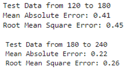
For each batch of test data, 120 to 180 and 180 to 240 will be the testing data to be fed into the trained model. Since we have 3 batches of test data, total of 6 tests will be performed. But in this article, only one batch of result will be shown.
for i in range(120,240,60):
    start = i
    end = start + n_steps_in
    last = end + n_steps_out
    y_pred_inv , dataset_test_y , past_data = prep_data(x1_test_scaled , x2_test_scaled , y_test , start , end , last)
    evaluate_prediction(y_pred_inv , dataset_test_y, 'LSTM' , start , end)
    plot_multistep(past_data , y_pred_inv , dataset_test_y , start , end)


Summary
In this tutorial, a LSTM model is developed. It has the capability of forecasting 30 steps ahead data based on previous 60 data with 2 features.
This code is also capable of processing datasets with more than 2 features
Feel free to modify the n_steps_in and n_steps_out for different variation.
Personal Note
Hopefully this article is able to help in understanding LSTM as well as the workflow of developing a RNN model. Also, this is my first article on Medium, do point out my mistakes for personal development.
Feel free to connect with me : LinkedIn
